![]()
Three Levels of ML Software
ML/AI is rapidly adopted by new applications and industries. As already been mentioned, the goal of a machine learning project is to build a statistical model by using collected data and applying machine learning algorithms. Yet building successful ML-based software projects is still difficult because every ML-based software needs to manage three main assets: Data, Model, and Code. Machine Learning Model Operationalization Management - MLOps, as a DevOps extension, establishes effective practices and processes around designing, building, and deploying ML models into production. We describe here essential technical methodologies, which are involved in the development of the Machine Learning-based software, namely Data Engineering, ML Model Engineering, and Software Release Engineering.
We recommend documenting everything you have learned in each step of the whole pipeline.
Data: Data Engineering Pipelines
We mentioned previously that the fundamental part of any machine learning workflow is Data. Collecting good data sets has a huge impact on the quality and performance of the ML model. The famous citation
“Garbage In, Garbage Out”,
in the machine learning context means that the ML model is only as good as your data. Therefore, the data, which has been used for training of the ML model, indirectly influence the overall performance of the production system. The amount and quality of the data set are usually problem-specific and can be empirically discovered.
Being an important step, data engineering is reported as heavily time-consuming. We might spend the majority of time on a machine learning project constructing data sets, cleaning, and transforming data.
The data engineering pipeline includes a sequence of operations on the available data. The final goal of these operations is to create training and testing datasets for the ML algorithms. In the following, we describe each stage of the data engineering pipeline such as Data Ingestion, Exploration and Validation, Data Wrangling (Cleaning), and Data Splitting.
Data Ingestion
Data Ingestion - Collecting data by using various systems, frameworks and formats, such as internal/external databases, data marts, OLAP cubes, data warehouses, OLTP systems, Spark, HDFS etc. This step might also include synthetic data generation or data enrichment The best practices for this step include the following actions that should be maximally automated:
- Data Sources Identification: Find the data and document its origin (data provenance).
- Space Estimation: Check how much storage space it will take.
- Space Location: Create a workspace with enough storage space.
- Obtaining Data: Get the data and convert them to a format that can be easily manipulated without changing the data itself.
- Back up Data: Always work on a copy of the data and keep the original dataset untouched.
- Privacy Compliance: Ensure sensitive information is deleted or protected (e.g., anonymized) to ensure GDPR compliance.
- Metadata Catalog: Start documenting the metadata of the dataset by recording the basic information about the size, format, aliases, last modified time, and access control lists. (Further reading)
- Test Data: Sample a test set, put it aside, and never look at it to avoid the “data snooping” bias. You fell for this if you are selecting a particular kind of ML model by using the test set. This will lead to an ML model selection that is too optimistic and will not perform well in production.
Exploration and Validation
Exploration and Validation - Includes data profiling to obtain information about the content and structure of the data. The output of this step is a set of metadata, such as max, min, avg of values. Data validation operations are user-defined error detection functions, which scan the dataset to spot some errors. The validation is a process of assessing the quality of the data by running dataset validation routines (error detection methods). For example, for “address”-attributes, are the address components consistent? Is the correct postal code associated with the address? Are there missing values in the relevant attributes? The best practices for this step include the following actions:
- Use RAD tools: Using Jupyter notebooks is a good way to keep records of data exploration and experimentation.
- Attribute Profiling: Obtain and document the metadata about each attribute, such as
- Name
- Number of Records
- Data Type (categorical, numerical, int/float, text, structured, etc.)
- Numerical Measures (min, max, avg, median, etc. for numerical data)
- Amount of missing values (or “missing value ratio” = Number of absent values/ Number of records)
- Type of distribution (Gaussian, uniform, logarithmic, etc.)
- Label Attribute Identification: For supervised learning tasks, identify the target attribute(s).
- Data Visualization: Build a visual representation for value distribution.
- Attributes Correlation: Compute and analyze the correlations between attributes.
- Additional Data: Identify data that would be useful for building the model (go back to “Data Ingestion”).
Data Wrangling (Cleaning)
Data Wrangling (Cleaning) - Data preparation step where we programmatically wrangle data, e.g., by re-formatting or re-structuring particular attributes that might change the form of the data’s schema. We recommend writing scripts or functions for all data transformations in the data pipeline to re-use all these functionalities on future data.
- Transformations: Identify the promising transformations you may want to apply.
- Outliers: Fix or remove outliers (optional).
- Missing Values: Fill in missing values (e.g., with zero, mean, median) or drop their rows or columns.
- Not relevant Data: Drop the attributes that provide no useful information for the task (relevant for feature engineering).
- Restructure Data: Might include the following operations (from the book “Principles of Data Wrangling”)
- Reordering record fields by moving columns
- Creating new record fields through extracting values
- Combining multiple record fields into a single record field
- Filtering datasets by removing sets of records
- Shifting the granularity of the dataset and the fields associated with records through aggregations and pivots.
Data Splitting
Data Splitting - Splitting the data into training (80 %), validation, and test datasets to be used during the core machine learning stages to produce the ML model.
Model: Machine Learning Pipelines
The core of the ML workflow is the phase of writing and executing machine learning algorithms to obtain an ML model. The model engineering pipeline is usually utilized by a data science team and includes a number of operations that lead to a final model. These operations include Model Training, Model Evaluation, Model Testing, and Model Packaging. We recommend automating these steps as much as possible.
Model Training
Model Training - The process of applying the machine learning algorithm on training data to train an ML model. It also includes feature engineering the hyperparameter tuning for the model training activity. The following list is adopted from “Hands-On Machine Learning with Scikit-Learn, Keras, and TensorFlow” by Aurélien Géron
-
Feature engineering might include:
- Discretize continuous features
- Decompose features (e.g., categorical, date/time, etc.)
- Add transformations of features (e.g., log(x), sqrt(x), x2, etc.)
- Aggregate features into promising new features
- Feature scaling: Standardize or normalize features
- New features should be added quickly to get fast from a feature idea to the feature running in production. Further reading “Feature Engineering for Machine Learning. Principles and Techniques for Data Scientists” by Alice Zheng, Amanda Casari
-
Model Engineering might be an iterative process and include the following workflow:
- Every ML model specification (code that creates an ML model) should go through a code review and be versioned.
- Train many ML models from different categories (e.g., linear regression, logistic regression, k-means, naive Bayes, SVM, Random Forest, etc.) using standard parameters.
- Measure and compare their performance. For each model, use N-fold cross-validation and compute the mean and standard deviation of the performance measure on the N folds.
- Error Analysis: analyze the types of errors the ML models make.
- Consider further feature selection and engineering.
- Identify the top three to five most promising models, preferring models that make different types of errors.
- Hyperparameters tuning by using cross-validation. Please note that data transformation choices are also hyperparameters. Random search for hyperparameters is preferred over grid search.
- Consider Ensemble methods such as majority vote, bagging, boosting, or stacking. Combining ML models should produce better performance than running them individually. (Further reading “Ensemble Methods: Foundations and Algorithms” by Zhi-Hua Zhou)
Model Evaluation
Model Evaluation - Validate the trained model to ensure it meets original business objectives before serving the ML model in production to the end-user.
Model Testing
Model Testing - Once the final ML model is trained, its performance needs to be measured by using the hold-back test dataset to estimate the generalization error by performing the final “Model Acceptance Test”.
Model Packaging
Model Packaging - The process of exporting the final ML model into a specific format (e.g. PMML, PFA, or ONNX), which describes the model to be consumed by the business application. We cover the ML model packaging in the part ‘ML Model serialization formats’ below.
Different forms of ML workflows
Operating an ML model might assume several architectural styles. In the following, we discuss four architectural patterns which are classified along two dimensions:
1. ML Model Training and
2. ML Model Prediction
Please note that for the sake of simplicity, we disregard the third dimension 3. ML Model Type, which denotes the type of machine learning algorithm such as supervised, unsupervised, semisupervised, and Reinforcement Learning.
There are two ways how we perform ML Model Training:
- Offline learning (aka batch or static learning): The model is trained on a set of already collected data. After deploying to the production environment, the ML model remains constant until it re-trained because the model will see a lot of real-live data and becomes stale. This phenomenon is called ‘model decay’ and should be carefully monitored.
- Online learning (aka dynamic learning): The model is regularly being re-trained as new data arrives, e.g. as data streams. This is usually the case for ML systems that use time-series data, such as sensor, or stock trading data to accommodate the temporal effects in the ML model.
The second dimension is ML Model Prediction, which denotes the mechanics of the ML model to makes predictions. Here we also distinguish two modes:
- Batch predictions: The deployed ML model makes a set of predictions based on historical input data. This is often sufficient for data that is not time-dependent, or when it is not critical to obtain real-time predictions as output.
- Real-time predictions (aka on-demand predictions): Predictions are generated in real-time using the input data that is available at the time of the request.
After identifying these two dimensions, we can classify the operationalization of machine learning models into four ML architecture patterns:
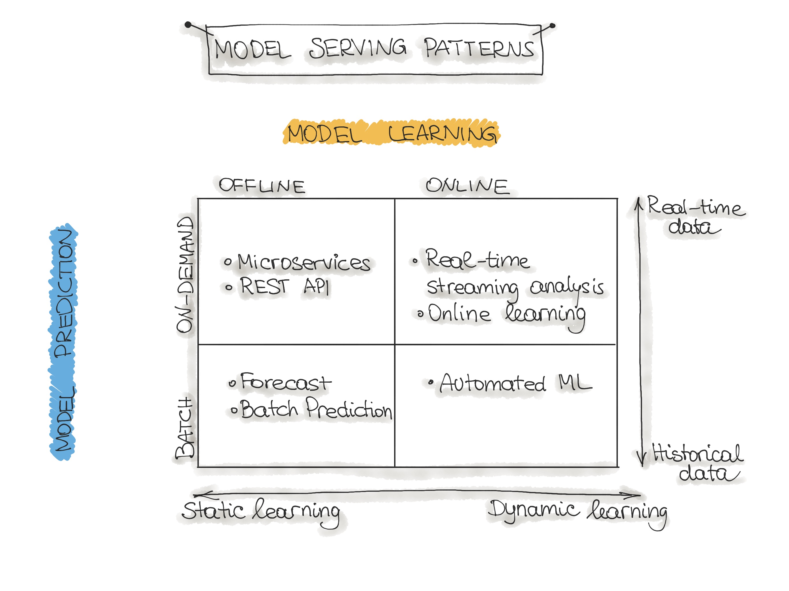
In the following, we present a description of the model architectural patterns such as Forecast, Web-Service, Online Learning, and AutoML.
Forecast
This type of machine learning workflow is widely spread in academic research or data science education (e.g., Kaggle or DataCamp). This form is used to experiment with ML algorithms and data as it is the easiest way to create a machine learning system. Usually, we take an available dataset, train the ML model, then run this model on another (mostly historical) data, and the ML model makes predictions. This way, we output a forecast. This ML workflow is not very useful and, therefore, not common in an industry setting for production systems (e.g. mobile applications).
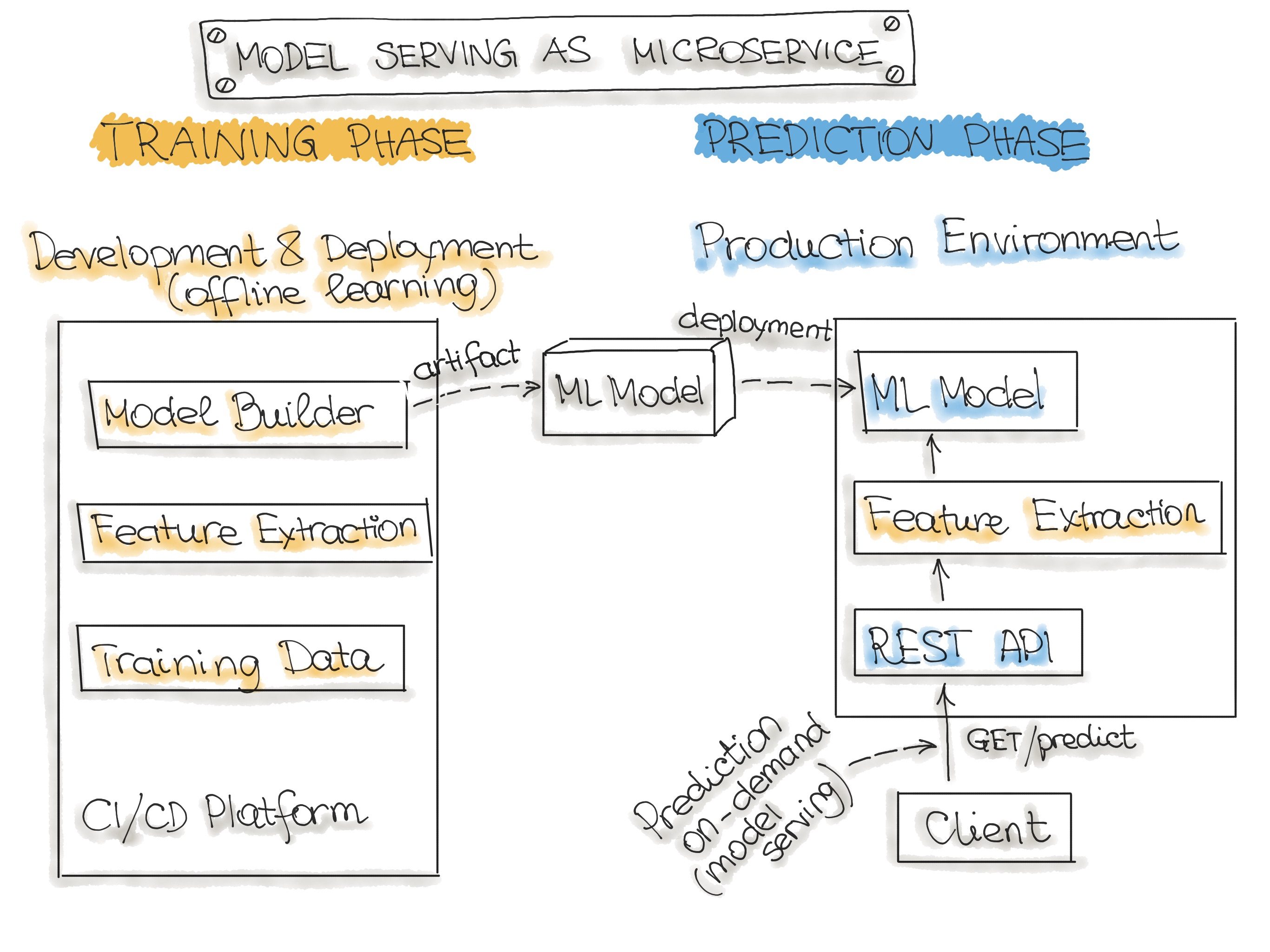
Web-Service
The most commonly described deployment architecture for ML models is a web service (microservise). The web service takes input data and outputs a prediction for the input data points. The model is trained offline on historical data, but it uses real-live data to make predictions. The difference from a forecast (batch predictions) is that the ML model runs near real-time and handles a single record at a time instead of processing all the data at once. The web service uses real-time data to make predictions, but the model remains constant until it is re-trained and re-deployed into the production system.
The figure below illustrates the architecture for wrapping trained models as deployable services. Please note, we discuss methods for wrapping trained ML models as deployable services in the Deployment Strategies Section.
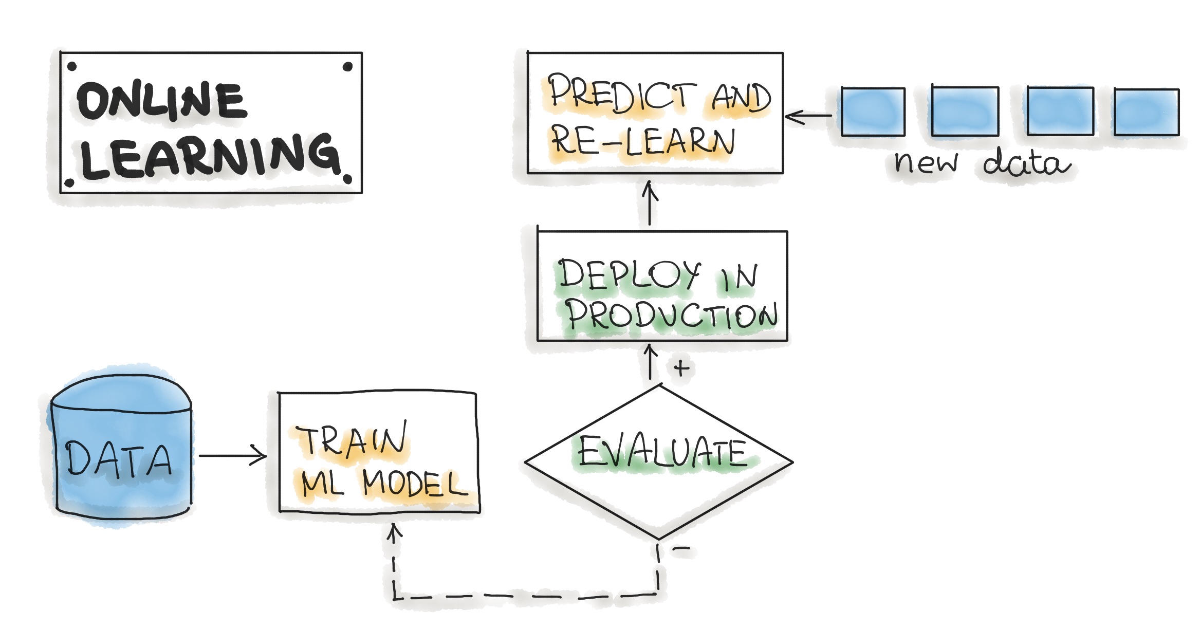
Online Learning
The most dynamic way to embed machine learning into a production system is to implement online learning, which is also known as real-time streaming analytics. Please note that online learning can be a confusing name because the core learning or ML model training is usually not performed on the live system. We should call it incremental learning; however, the term online learning is already established within the ML community.
In this type of ML workflow, the ML learning algorithm is continuously receiving a data stream, either as single data points or in small groups called mini-batches. The system learns about new data on the fly as it arrives, so the ML model is incrementally being re-trained with new data. This continually re-trained model is instantly available as a web service.
Technically, this type of ML system works well with the lambda architecture in big data systems. Usually, the input data is a stream of events, and the ML model takes the data as it enters the system, provides predictions and re-learns on these new data. The model would typically run as a service on a Kubernetes cluster or similar.
A big difficulty with the online learning system in production is that if bad data is entering the system, the ML model, as well as the whole system performance, will increasingly decline.
AutoML
An even more sophisticated version of online learning is automated machine learning or AutoML.
AutoML is getting a lot of attention and is considered the next advance for enterprise ML. AutoML promises training ML models with minimal effort and without machine learning expertise. The user needs to provide data, and the AutoML system automatically selects an ML algorithm, such as neural network architecture, and configures the selected algorithm.
Instead of updating the model, we execute an entire ML model training pipeline in production that results in new models on the fly. For now, this is a very experimental way to implement ML workflows. AutoML is usually provided by big cloud providers, such as Google or MS Azure. However, models build with AutoML need to reach the level of accuracy required for real-world success.
Further reading
ML Model serialization formats
There are various formats to distribute ML models. In order to achieve a distributable format, the ML model should be present and should be executable as an independent asset. For example, we might want to use a Scikit-learn model in a Spark job. This means that the ML models should work outside of the model-training environment. In the following, we describe Language-agnostic and Vendor-specific exchange formats for ML models.
Language-agnostic exchange formats
- Amalgamation is the simplest way to export an ML model. The model and all necessary code to run are bundled as one package. Usually, it is a single source code file that can be compiled on nearly any platform as a standalone program. For example, we can create a standalone version of an ML model by using SKompiler. This python package provides a tool for transforming trained Scikit-learn models into other forms, such as SQL queries, Excel formulas, Portable Format for Analytics (PFA) files, or SymPy expressions. The last can be translated to code in a variety of languages, such as C, Javascript, Rust, Julia, etc. Amalgamation is a straightforward concept, and the exported ML models are portable. With some easy ML algorithms, such as logistic regression or decision tree, this format is compact and might have good performance, which is useful for constrained embedded environments. However, the ML model code and parameters need to be managed together.
- PMML is a format for model serving based on XML with the file extension .pmml. PMML has been standardized by the Data Mining Group (DMG). Basically, .ppml describes a model and pipeline in XML. The PMML supports not all of the ML algorithms, and its usage in open source-driven tools is limited due to licensing issues.
- PFA (Portable Format for Analytics) is designed as a replacement for PMML. From DMG: “A PFA document is a string of JSON-formatted text that describes an executable called a scoring engine. Each engine has a well-defined input, a well-defined output, and functions for combining inputs to construct the output in an expression-centric syntax tree”. PFA capabilities include (1) control structures, such as conditionals, loops, and user-defined functions, (2) expressed within JSON, and can, therefore, be easily generated and manipulated by other programs, (3) fine-grained function library supporting extensibility callbacks. To run ML models as PFA files, we will need a PFA-enabled environment.
- ONNX (Open Neural Network eXchange) is an ML framework independent file format. ONNX was created to allow any ML tool to share a single model format. This format is supported by many big tech companies such as Microsoft, Facebook, and Amazon. Once the ML model is serialized in the ONNX format, it can be consumed by onnx-enabled runtime libraries (also called inference engines) and then make predictions. Here you will find the list of tools that can use ONNX format. Notably that most deep learning tools have ONNX support.
Vendor-specific exchange formats
- Scikit-Learn saves models as pickled python objects, with a .pkl file extension.
- H2O allows you to convert the models you have built to either POJO (Plain Old Java Object) or MOJO (Model Object, Optimized).
- SparkML models that can be saved in the MLeap file format and served in real-time using an MLeap model server. The MLeap runtime is a JAR that can run in any Java application.MLeap supports Spark, Scikit-learn, and Tensorflow for training pipelines and exporting them to an MLeap Bundle.
- TensorFlow saves models as .pb files; which is the protocol buffer files extension.
- PyTorch serves models by using their proprietary Torch Script as a .pt file. Their model format can be served from a C– application.
- Keras saves a model as a .h5 file, which is known in the scientific community as a data file saved in the Hierarchical Data Format (HDF). This type of file contains multidimensional arrays of data.
- Apple has its proprietary file format with the extension .mlmodel to store models embedded in iOS applications. The Core ML framework has native support for Objective-C and Swift programming languages. Applications trained in other ML frameworks, such as TensorFlow, Scikit-Learn, and other frameworks need to use tools like such as coremltools and Tensorflow converter to translate their ML model files to the .mlmodel format for use on iOS.
The following Table summarizes all ML model serialization formats:
| Open-Format | Vendor | File Extension | License | ML Tools & Platforms Support | Human-readable | Compression | |
|---|---|---|---|---|---|---|---|
| "almagination" | − | − | − | − | − | − | ✓ |
| PMML | ✓ | DMG | .pmml | AGPL | R, Python, Spark | ✓ (XML) | ✘ |
| PFA | ✓ | DMG | JSON | PFA-enabled runtime | ✓ (JSON) | ✘ | |
| ONNX | ✓ | SIG LFAI |
.onnx | TF, CNTK, Core ML, MXNet, ML.NET | − | ✓ | |
| TF Serving Format | ✓ | .pf | Tensor Flow | ✘ | g-zip | ||
| Pickle Format | ✓ | .pkl | scikit-learn | ✘ | g-zip | ||
| JAR/ POJO | ✓ | .jar | H2O | ✘ | ✓ | ||
| HDF | ✓ | .h5 | Keras | ✘ | ✓ | ||
| MLEAP | ✓ | .jar/ .zip | Spark, TF, scikit-learn | ✘ | g-zip | ||
| Torch Script | ✘ | .pt | PyTorch | ✘ | ✓ | ||
| Apple .mlmodel | ✘ | Apple | .mlmodel | TensorFlow, scikit-learn, Core ML | − | ✓ |
Further reading:
Code: Deployment Pipelines
The final stage of delivering an ML project includes the following three steps:
- Model Serving - The process of deploying the ML model in a production environment.
- Model Performance Monitoring - The process of observing the ML model performance based on live and previously unseen data, such as prediction or recommendation. In particular, we are interested in ML-specific signals, such as prediction deviation from previous model performance. These signals might be used as triggers for model re-training.
- Model Performance Logging - Every inference request results in a log-record.
In the following, we discuss Model Serving Patterns and Model Deployment Strategies.
Model Serving Patterns
Three components should be considered when we serve an ML model in a production environment. The inference is the process of getting data to be ingested by a model to compute predictions. This process requires a model, an interpreter for the execution, and input data.
Deploying an ML system to a production environment includes two aspects, first deploying the pipeline for automated retraining and ML model deployment. Second, providing the API for prediction on unseen data.
Model serving is a way to integrate the ML model in a software system. We distinguish between five patterns to put the ML model in production: Model-as-Service, Model-as-Dependency, Precompute, Model-on-Demand, and Hybrid-Serving. Please note that the above-described model serialization formats might be used for any of the model serving patterns.
The following taxonomy shows these approaches:
| Machine Learning Model Serving Taxonomy | |||
|---|---|---|---|
| ML Model | |||
| Service & Versioning | Together with the consuming application | Independent from the consuming application | |
| Compile/ Runtime Availabilty | Build & runtime available | Available remotely through REST API/RPC | Available at the runtime scope |
| Serving Patterns | "Model-as-Dependency" | "Model-as-Service" | "Precompute" and "Model on Demand" |
| Hybrid Model Serving (Federated Learning) | |||
Now, we present the serving patterns to productionize the ML model such as Model-as-Service, Model-as-Dependency, Precompute, Model-on-Demand, and Hybrid-Serving.
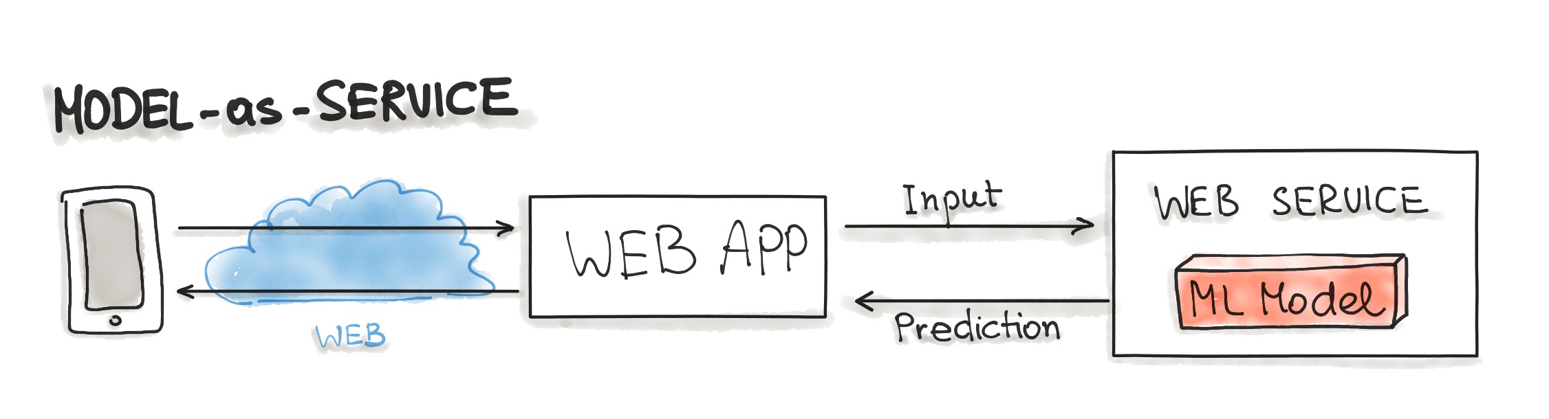
Model-as-Service
Model-as-Service is a common pattern for wrapping an ML model as an independent service. We can wrap the ML model and the interpreter within a dedicated web service that applications can request through a REST API or consume as a gRPC service.
This pattern can be used for various ML workflows, such as Forecast, Web Service, Online Learning.
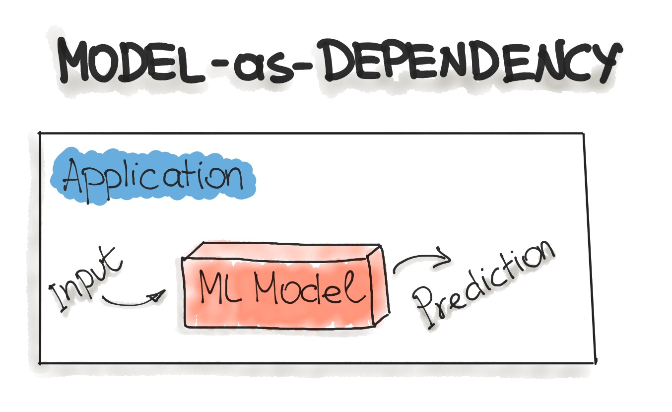
Model-as-Dependency
Model-as-Dependency is probably the most straightforward way to package an ML model. A packaged ML model is considered as a dependency within the software application. For example, the application consumes the ML model like a conventional jar dependency by invoking the prediction method and passing the values. The return value of such method execution is some prediction that is performed by the previously trained ML model. The Model-as-Dependency approach is mostly used for implementing the Forecast pattern.
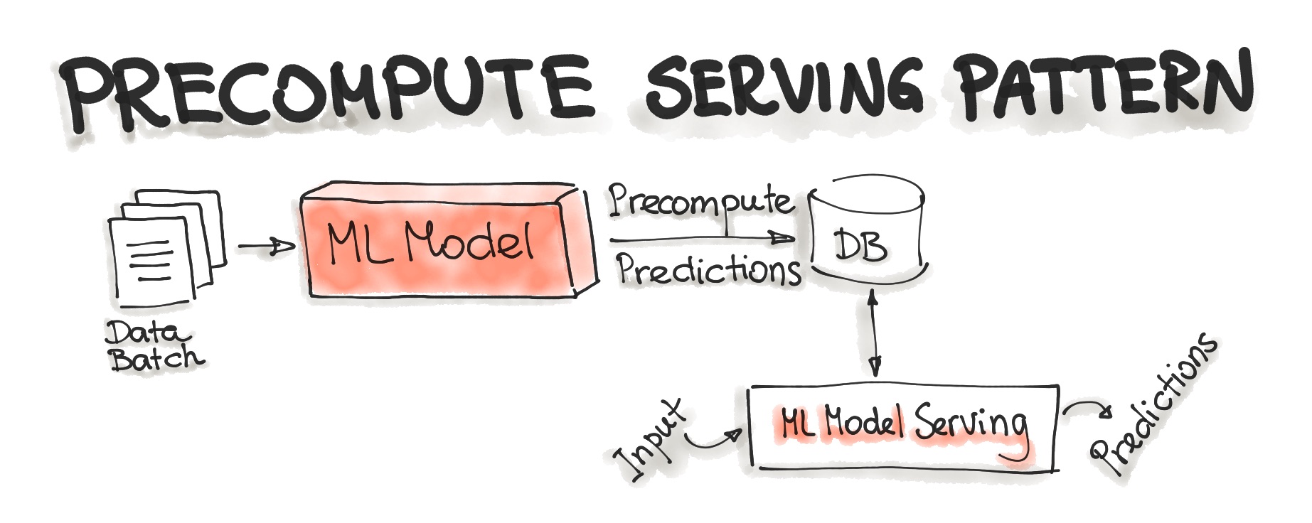
Precompute Serving Pattern
This type of ML model serving is tightly related to the Forecast ML workflow. With the Precompute serving pattern, we use an already trained ML model and precompute the predictions for the incoming batch of data. The resulting predictions are persisted in the database. Therefore, for any input request, we query the database to get the prediction result.
Further reading: Bringing ML to Production (Slides)
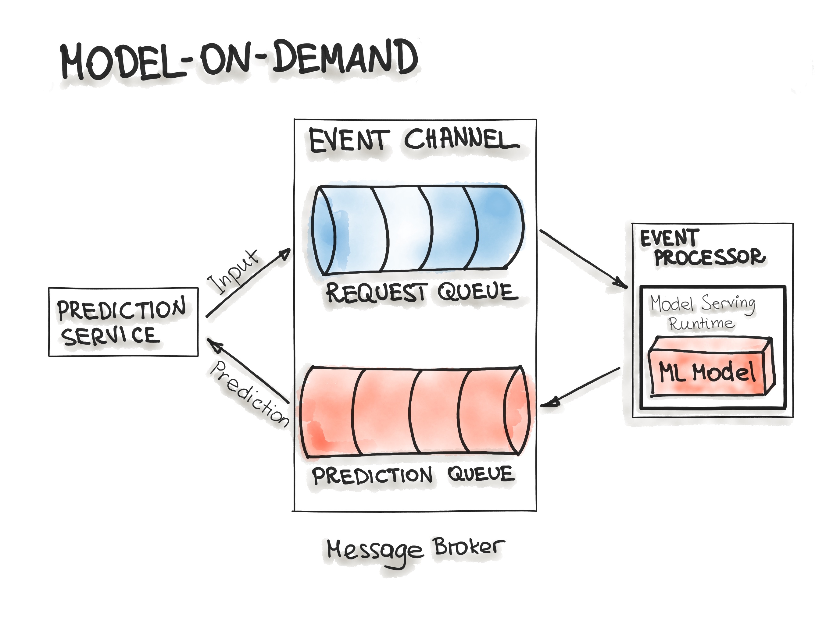
Model-on-Demand
The Model-on-Demand pattern also treats the ML model as a dependency that is available at runtime. This ML model, contrary to the Model-as-Dependency pattern, has its own release cycle and is published independently.
The message-broker architecture is typically used for such on-demand model serving. The message-broker topology architecture pattern contains two main types of architecture components: a broker component and an event processor component. The broker component is the central part that contains the event channels that are utilised within the event flow. The event channels, which are enclosed in the broker component, are message queues. We can imagine such architecture containing input- and output-queues. A message broker allows one process to write prediction-requests in an input queue. The event processor contains the model serving runtime and the ML model. This process connects to the broker, reads these requests in batch from the queue and sends them to the model to make the predictions. The model serving process runs the prediction generation on the input data and writes the resulted predictions to the output queue. Afterwards, the queued prediction results are pushed to the prediction service that initiated the prediction request.
Further reading:
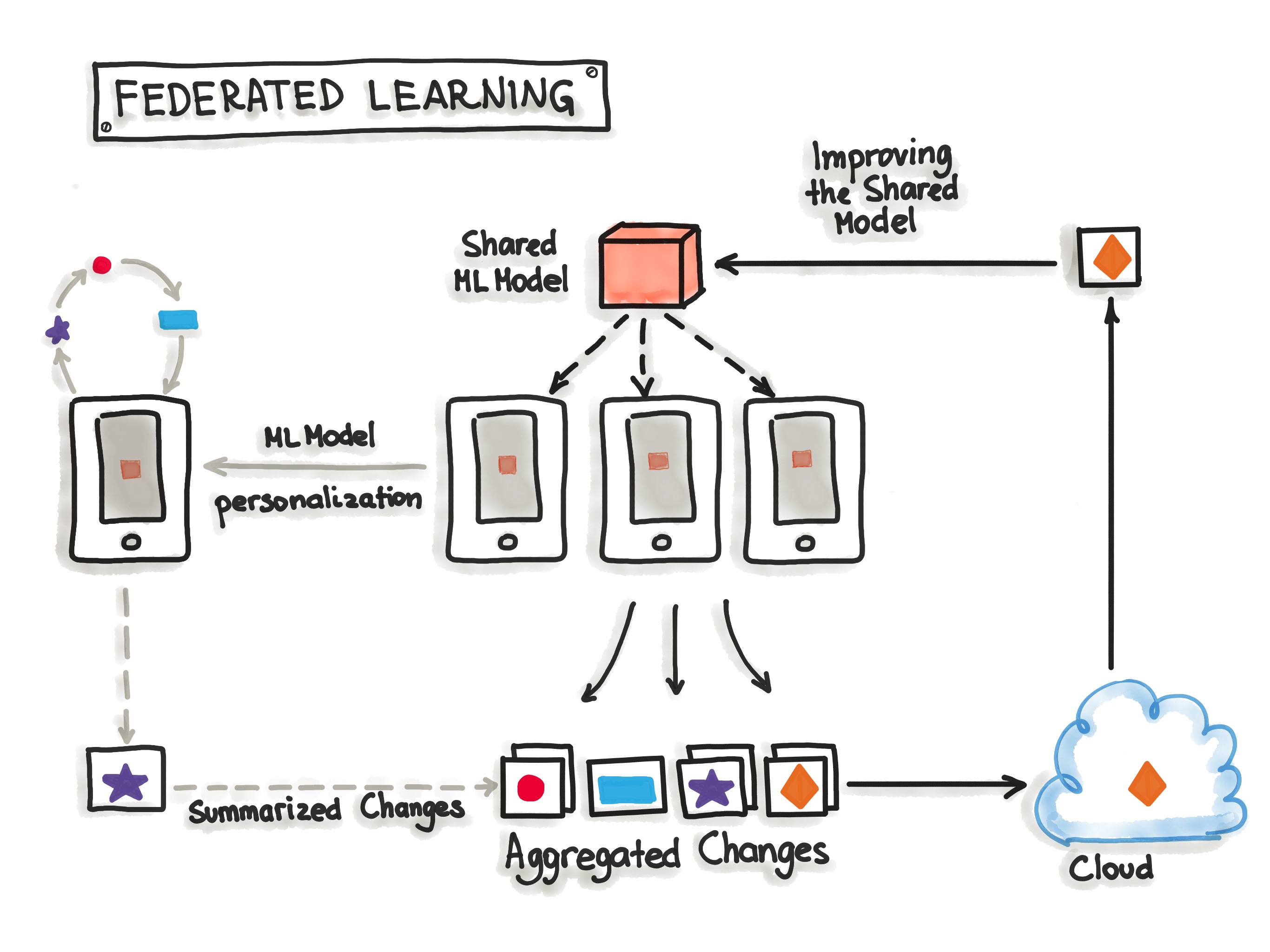
Hybrid-Serving (Federated Learning)
Federated Learning, also known as hybrid-serving, is another way of serving a model to the users. It is unique in the way it does, there is not only one model that predicts the outcome, but there are also lots of it. Exactly spoken there are as many models as users exist, in addition to the one that’s held on a server. Let us start with the unique model, the one on the server. The model on the server-side is trained only once with the real-world data. It sets the initial model for each user. Also, it is a relatively general trained model so it fits for the majority of users. On the other side, there are the user-side models, which are the real unique models. Due to the raising hardware standards on mobile devices, it is possible for the devices to train their own models. Like that the devices will train their own highly specialized model for their own user. Once in a while, the devices send their already trained model data (not the personal data) to the server. There the server model will be adjusted, so the actual trends of the whole user community will be covered by the model. This model is set to be the new initial model that all devices are using. For not having any downsides for the users, while the server model gets updated, this happens only when the device is idle, connected to WiFi and charging. Also, the testing is done on the devices, therefore the newly adopted model from the server is sent to the devices and tested for functionality.
The big benefit of this is that the data used for training and testing, which is highly personal, never leaves the devices while still capturing all data that is available. This way it is possible to train highly accurate models while not having to store tons of (probably personal) data in the cloud. But there is no such thing as a free lunch, normal machine learning algorithms are built with homogeneously and large datasets on powerful hardware which is always available for training. With Federated Learning there are other circumstances, the mobile devices are less powerful, the training data is distributed across millions of devices and these are not always available for training. Exactly for this TensorFlow Federated (TFF) has been created. TFF is a lightweight form of TensorFlow created for Federated Learning.
Deployment Strategies
In the following, we discuss common ways for wrapping trained models as deployable services, namely deploying ML models as Docker Containers to Cloud Instances and as Serverless Functions.
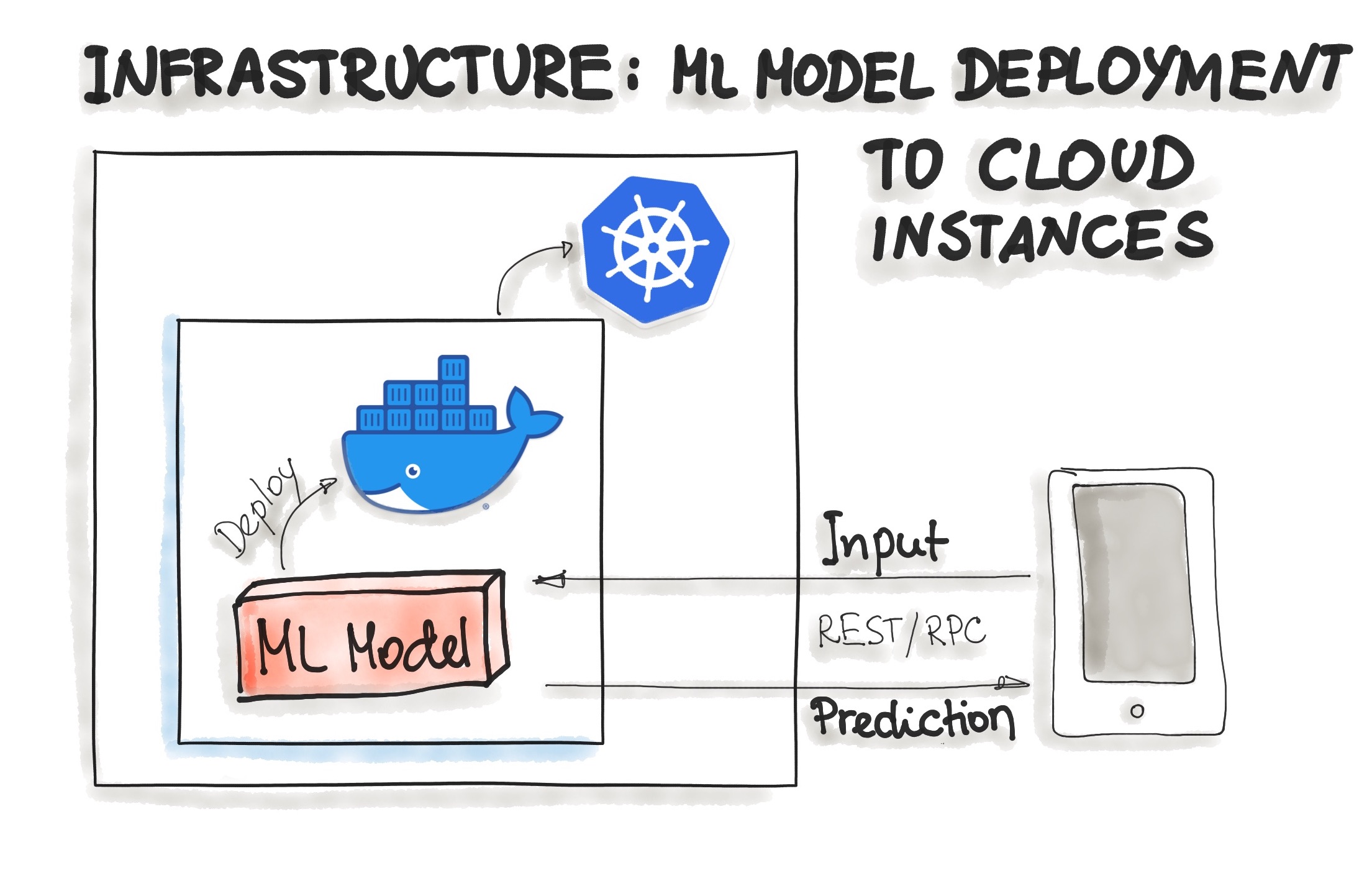
Deploying ML Models as Docker Containers
As of now, there is no standard, open solution to ML model deployment. As ML model inference being considered stateless, lightweight, and idempotent, containerization becomes the de-facto standard for delivery. This means we deploy a container that wraps an ML model inference code. For on-premise, cloud, or hybrid deployments, Docker is considered to be de-facto standard containerization technology.
One ubiquitous way is to package the whole ML tech stack (dependencies) and the code for ML model prediction into a Docker container. Then Kubernetes or an alternative (e.g. AWS Fargate) does the orchestration. The ML model functionality, such as prediction, is then available through a REST API (e.g. implemented as Flask application)
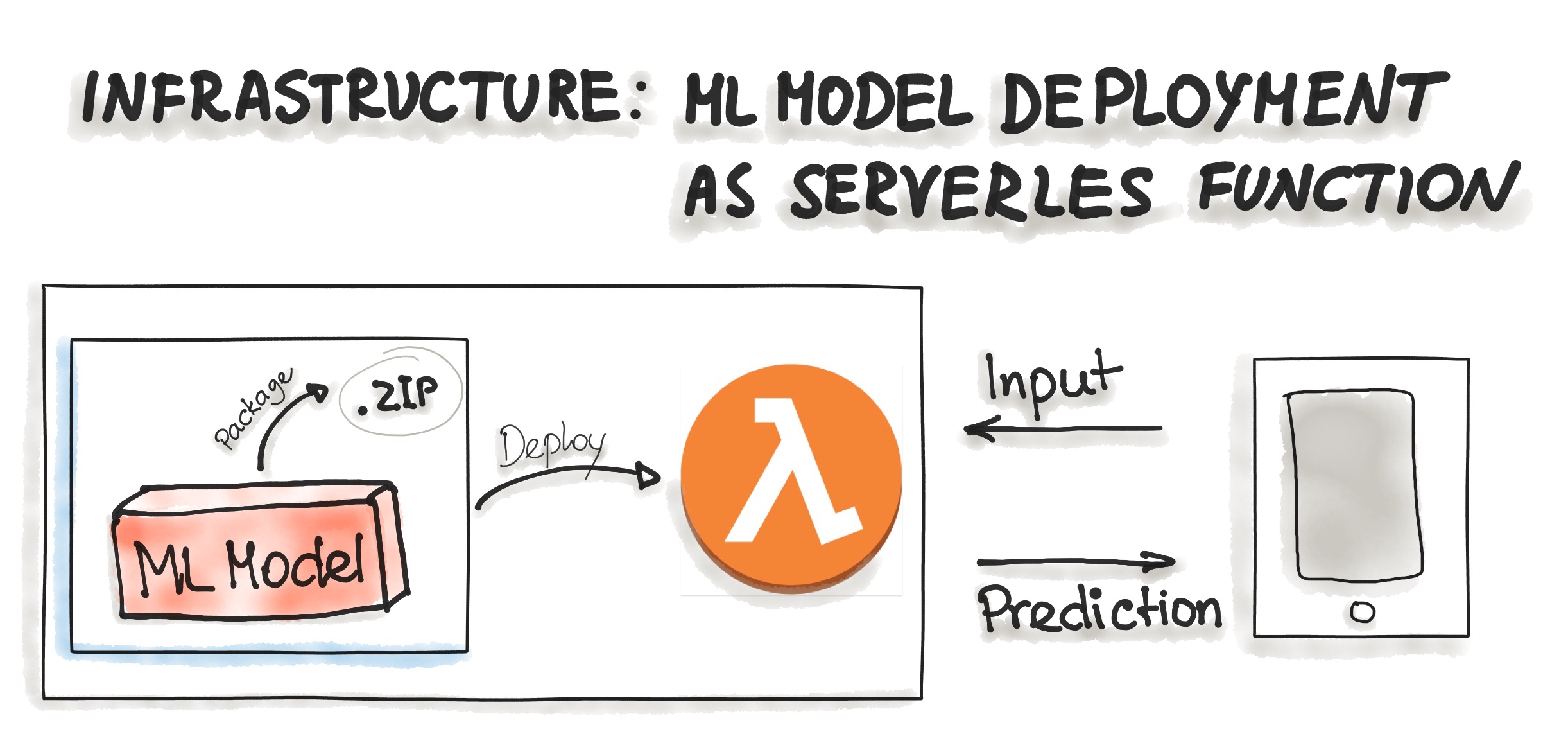
Deploying ML Models as Serverless Functions
Various cloud vendors already provide machine-learning platforms, and you can deploy your model with their services. Examples are Amazon AWS Sagemaker, Google Cloud AI Platform, Azure Machine Learning Studio, and IBM Watson Machine Learning, to name a few. Commercial cloud services also provide containerization of ML models such as AWS Lambda and Google App Engine servlet host.
In order to deploy an ML model as a serverless function, the application code and dependencies are packaged into .zip files, with a single entry point function. This function then could be managed by major cloud providers such as Azure Functions, AWS Lambda, or Google Cloud Functions. However, attention should be paid to possible constraints of the deployed artifacts such as the size of the artifact.